This blog post is for the newbies who want to quickly understand the basics of the most popular Machine Learning algorithms. I am assuming that you have read the previous article regarding types or categories of algorithms. If not, I would suggest you to read that first.
In this quick tour you will learn about:
- Linear Regression
- Logistic Regression
- Decision Trees
- Naive Bayes
- Support Vector Machines, SVM
- K-Nearest Neighbors, KNN
- K-Means
- Random Forest
- Dimensionality Reduction
- Artificial Neural Networks, ANN
Let’s get started!
1. Linear Regression
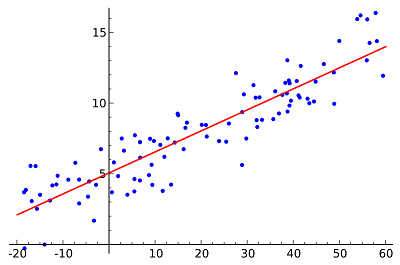
Linear Regression is one of the most (or probably “the most”) popular Machine Learning algorithms. Remember when in high school you had to plot data points on a graph (given X axis and Y axis) and then find the line of best fit? That is a very simple Machine Learning algorithm. In more technical terms, linear regression attempts to establish a relationship between one or more independent variables (points on X axis) and a numeric outcome or dependent variable (value on Y axis) by fitting the equation of a line to observed data:
Y = a*X + b
For example, you might want to relate the weights (Y) of individuals to their heights (X) using linear regression. This approach assumes a strong linear relationship between input and output variables — we would assume that if height increases then weight also increases proportionally in a linear way.
The goal here is to derive optimal values for a and b so that our estimated values, Y, can be as close as possible to their correct values (we know the actual values for Y at this stage because we are trying to learn our equation from the examples given in the training data set).
Once our Machine Learning model has learnt the line of best fit via Linear Regression, this line can then be used to predict values for new or unseen data points.
Different techniques can be used to learn the linear regression model, i.e., to derive the optimal values for the coefficients a and b. The two most popular methods:
- Ordinary least squares: The method of least squares calculates the best-fitting line by minimizing the vertical distances from each data point to the line. If a point lies on the fitted line exactly then its vertical distance from the line is 0. More specifically, the overall distance is the sum of the squares of the vertical distances for all the data points. The idea is to fit a model by minimizing this squared error or distance — blue points as close as possible to the red line.
- Gradient descent is a method that minimizes the amount of error at each step of the model training process. You can read more about its inner workings here.
When we are dealing with only one independent variable, like in the figure above, then we call it Simple Linear Regression. When there are more than one independent variables (e.g., we want to predict weight using more variables than just the person’s height) then this type of regression is termed as Multiple Linear Regression. Also, while finding the line of best fit, you can use a polynomial (a curved line) instead of a straight line — polynomial regression.
2. Logistic Regression
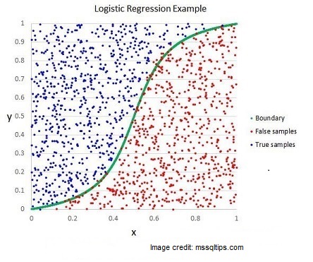
Logistic Regression has the same main idea as linear regression. The difference is that this technique is used when the output or dependent variable is binary — the outcome can have only two possible values. For example, let’s say that we want to predict if age has an influence on the probability of having a heart attack. In this case, our prediction needs only be a “yes” or “no” answer — only two possible values.
In logistic regression, the line of best fit is not a straight line anymore. The prediction for the final output is transformed using a non-linear S-shaped function called the logistic function, g(). This logistic function maps the intermediate outcome values into an outcome variable Y with values ranging from 0 to 1. These 0 to 1 values can then be interpreted as the probability of occurrence of Y. In the heart attack example, we have two class labels to be predicted (“yes” as 1 and “no” as 0). If we set a threshold of 0.5 then all the instances with a probability higher than the threshold will be classified as instances belonging to class 1 (“yes”) while all those having probability below the threshold will be assigned to class 0 (“no”). In other words, the properties of the S-shaped logistic function make logistic regression suitable for classification tasks.
3. Decision Trees
Decision Trees belongs to the category of supervised learning algorithms. They can be used for solving both regression and classification tasks.
In this algorithm, the training model learns to predict values of the target variable by learning decision rules and a tree representation. A tree is made up of nodes corresponding to a feature or attribute. At each node we ask a question about the data. The left and right branches represent the possible answers. The final nodes, leaf nodes, correspond to a class label/predicted value. The importance for each feature is determined in a top-down approach — the higher the node, the more important its attribute/feature. This is more easy to understand by a visual representation of an example problem:
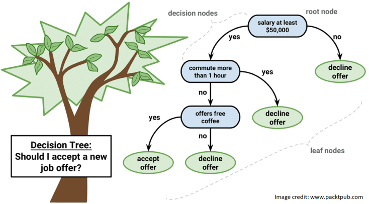
In the image above, you can see that data instances are classified into “will accept the offer or not” based on attributes like salary range and commute time. Salary is at a higher node than “offers free-coffee” implying that it is more important in determining the final outcome.
4. Naive Bayes
Naive Bayes is a simple and widely used Machine Learning algorithm based on the Bayes Theorem — remember your statistics lectures from high school/college? It is called naive because the classifier assumes that the input variables are independent of each other (a strong and unrealistic assumption for real data). The Bayes theorem is given by the equation below:
P(c|x) = P(x|c) . P(c) / P(x)
where, P(c|x) is the probability of the event of class c, given the predictor x; P(x|c) is the probability of x, given c; P(c) is the probability of the class; P(x) is the probability of the predictor. To put it simply, the model is composed of two types of probabilities:
- The probability of each class;
- The conditional probability for each class given each value of x
Let’s say we have a training data set of weather conditions (x) and corresponding target variable “Play” (c). We might want to obtain the probability of “Players will play if it is rainy”, P(c|x) . (Even if the answer is a numerical value ranging from 0 to 1, this is a classification problem — we can use the probabilities to reach a yes/no outcome.)
5. Support Vector Machine, SVM
Support Vector Machines is a supervised Machine Learning algorithm, used mainly for classification problems. In this algorithm, we plot each data item as a point in n-dimensional space, where n is number of input features. For example, with two input variables, we would have a two-dimensional space. Based on these transformations, SVM finds an optimal boundary, a hyperplane, that best separates the possible outputs by their class label. In a two-dimensional space, this hyperplane can be visualized as a line (not necessarily a straight line). The task of the SVM algorithm is to find the coefficients that provide the best separation of classes by this hyperplane.
The distance between the hyperplane (line) and the closest class points is called the margin. The optimal hyperplane is one that has the largest margin — one that classifies points in such a way that the distance between the closest data point from both classes is maximum.
In simple words, suppose you are given a plot of two classes (red and blue dots) on a graph as shown in the figure below. The job of the SVM classifier would be to decide the best line that can separate the blue dots from the red dots.
6. K-Nearest Neighbors, KNN
KNN algorithm is a very simple and popular technique. It is based on the following principle from real life: ‘You are the average of the five people you most associate with’!
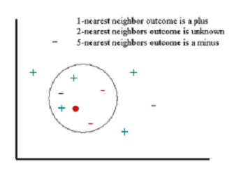
KNN classifies an object by searching through the entire training set for the K most similar instances (the K neighbors), and it assigns a common output variable to all those K instances. The figure below represents a classification example. If we classify a new instance (red circle) based on its 5 nearest neighbors, we would assign it to the “minus” category. But if we look only at its 1 nearest neighbor then it would end up in the “plus” category. Hence, the selection of K is critical here — a small value can result in a lot of noise and inaccurate results, while a large value is not feasible and defeats the purpose of the algorithm.
Although mostly used for classification, this technique can also be used for regression problems. For example, when dealing with a regression task, the output variable can be the mean of the K instances while for classification problems this can be the mode (or most common) class value.
The distance functions for assessing similarity between instances can be the so called Euclidean, Manhattan and Minkowski distances. Euclidean distance is simply an “ordinary” straight-line distance between two points (to be specific, the square root of the sum of the squares of the differences between corresponding coordinates of the points).
7. K-Means
K-means is a type of unsupervised algorithm for data clustering. It follows a simple procedure to classify a given data set — it tries to find K number of clusters or groups in the dataset. Since we are dealing with unsupervised learning, all we have is our training data X and the number of clusters K, but no labelled training instances (i.e., data with known final output category that we could use to train our model). For example, K-Means could be used to segment users into K groups based on their purchase history.
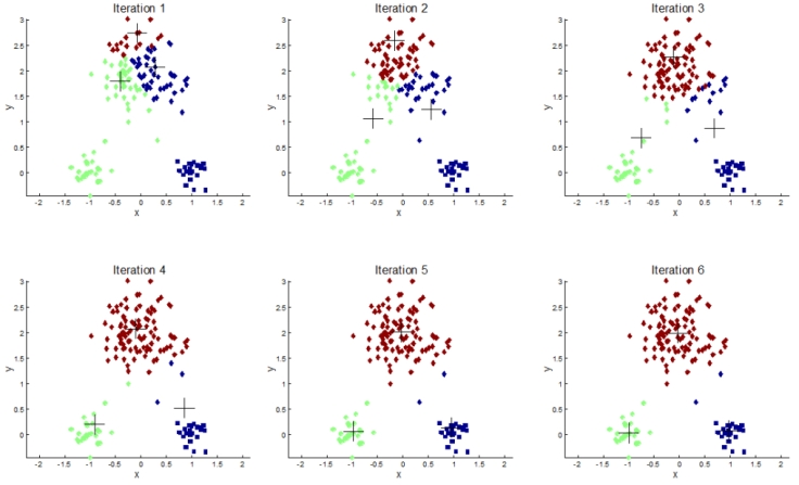
The algorithm iteratively assigns each data point to one of the K groups based on their features. Initially, it picks k points for each each of the K-clusters, known as the centroid. A new data point from the dataset is put into the cluster having the closest centroid based on feature similarity. As new elements are added to the cluster, the cluster centroid is recomputed and it keeps changing — the new centroid becomes the average location of all the data points currently in the cluster. This process is continued iteratively until the centroids stop changing. At the end, each centroid is a collection of feature values which define the resulting group.
Continuing with the purchase history example, the red cluster might represent users that like to buy tech gadgets and the blue one might be users interested in buying sports equipment. Now the algorithm will keep moving the centroid (“+” sign in the figure below) for each user-segment until it is able to create K groups. And it will do so by trying to maximize the separation between groups and users outside of the group.
8. Random Forest
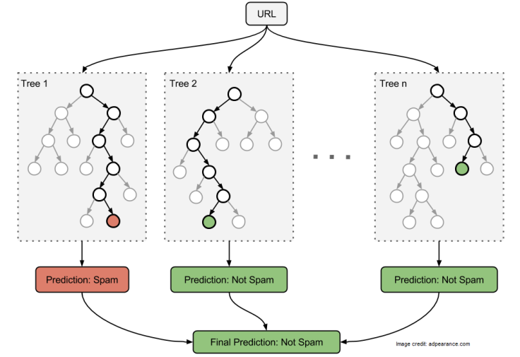
Random Forest is one of the most popular and powerful Machine Learning algorithms. It is a type of ensemble algorithm. The underlying idea for ensemble learning is “wisdom of crowds” — collective opinion of many is more likely to be accurate than that of one. The outcome of each of the models is combined and a prediction is made.
In Random Forest, we have an ensemble of decision trees (seen above, in algorithm 3). When we want to classify a new object, we take the vote of each decision tree and combine the outcome to make a final decision — majority vote wins.
9. Dimensionality Reduction
In the last years, there has been an exponential increase in the amount of data captured. This means that many Machine Learning problems involve thousands or even millions of features for each training instance. This makes not only training extremely slow, but finding a good solution also becomes much harder. This problem is often referred to as the curse of dimensionality. In real-world problems, it is often possible to reduce the number of features considerably, making problems tractable.
For example, in an image classification problem, if the pixels on the image borders are almost always white, these pixels can completely be dropped from the training set without losing much information.
Principal Component Analysis (PCA) is by far the most popular dimensionality reduction algorithm. PCA requires a blogpost on its own, so I will leave its details for some future post.
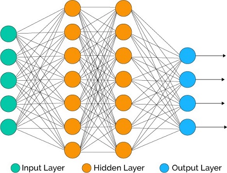
10. Artificial Neural Networks, ANN
Last but not the least, a sneak peek into Artificial Neural Networks which are at the very core of Deep Learning. ANN are ideal to tackle large and highly complex Machine Learning tasks, such as recommending the best videos to watch to hundreds of millions of users every day (e.g., YouTube), powering speech recognition services (e.g., Siri, Cortana) or learning to beat the world champion at the game of Go (DeepMind’s AlphaGo).
The key idea behind ANN is to use brain’s architecture for inspiration on how to build intelligent machines. ANN require a huge amount of training data, high computational power and long training time but, in the end, they are able make very accurate predictions.
To train a neural network, a set of neurons are mapped out and assigned a random weight which determines how the neurons process new data (images, text, sounds). The correct relationship between inputs and outputs is learned from training the neural network on input data. And since during the training phase the system gets to see the correct answers, if the network doesn’t accurately identify the input – doesn’t see a face in an image, for example — then the system adjusts the weights. Eventually, after sufficient training, the neural network will consistently recognize the correct patterns in speech, text or images.
So a neural network is a essentially a set of interconnected layers with weighted edges and nodes called neurons. Between the input and output layers you can insert multiple hidden layers. ANN make use of only two hidden layers. However, if we increase the depth of these layers then we are dealing with the famous Deep Learning.
End Notes
I hope that by now you have a very good overview of the most commonly used Machine Learning algorithms. The idea behind this post was to give you a high level walk-through. For details regarding each of these algorithms, stay tuned!
. . .
If you enjoyed reading this post and you want to continue on this Machine Learning journey, press the follow button to receive the latest right at your inbox!
